Get started easily going from basics to intermediate in data visualization with Python using Matplotlib and Seaborn. This tutorial covers some basic usage patterns and best practices to help you get started with Matplotlib and Seaborn. You will also be introduced to Exploratory Data Analysis (EDA) as a way to use data visualization to better understand your datasets. Understanding these foundational principles will help you create effective and insightful data visualizations that can inform and engage your audience.
import matplotlib as mpl

import matplotlib.pyplot as plt

import numpy as np
A simple example of data visualization with Python
Matplotlib graphs your data on Figures (e.g., windows, Jupyter widgets, etc.), each of which can contain one or more Axes, an area where points can be specified in terms of x-y coordinates (or theta-r in a polar plot, x-y-z in a 3D plot, etc). The simplest way of creating a Figure with an Axes is using pyplot.subplots. We can then use Axes.plot to draw some data on the Axes:
fig, ax = plt.subplots()  # Create a figure containing a single axes.

ax.plot([1, 2, 3, 4], [1, 4, 2, 3]);  # Plot some data on the axes.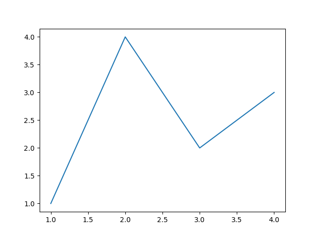
Key principles and steps to follow to perform the best data visualization
The foundations of data visualization involve understanding key principles and techniques to effectively communicate data insights. Here are some fundamental concepts:
- Know Your Audience: Tailor your visualizations to the knowledge level and interests of your audience.
- Choose the Right Chart Type:
- Bar Charts: For comparing quantities across categories.
- Line Charts: For showing trends over time.
- Scatter Plots: For showing relationships between two variables.
- Histograms: For showing the distribution of a single variable.
- Pie Charts: For showing parts of a whole (though often less effective than bar charts).
- Simplify: Keep the visualization as simple as possible to convey the message without unnecessary complexity.
- Use Appropriate Scales: Ensure that the scales used (e.g., linear, logarithmic) are appropriate for the data and context.
- Label Clearly: Axis labels, titles, and legends should be clear and descriptive to ensure the visualization is understandable.
- Use Color Wisely: Colors should enhance comprehension, not distract. Use color to highlight important information or to differentiate between data series.
- Highlight Key Points: Emphasize important data points or trends to guide the viewer’s attention.
- Maintain Proportions: Avoid distorting data by maintaining proper proportions in the visual representation.
- Consider Accessibility: Ensure visualizations are accessible to all users, including those with color vision deficiencies.
- Tell a Story: Use the visualization to tell a clear and compelling story about the data.
Parts of a Matplotlib Figure to Visualize Data
Here are the components of a Matplotlib Figure.

Pyplot Figure
The whole figure. The Figure keeps track of all the child Axes, a group of ‘special’ Artists (titles, figure legends, colorbars, etc), and even nested subfigures.
The easiest way to create a new Figure is with pyplot:
fig = plt.figure()  # an empty figure with no Axes

fig, ax = plt.subplots()  # a figure with a single Axes

fig, axs = plt.subplots(2, 2)  # a figure with a 2x2 grid of Axes
It is often convenient to create the Axes together with the Figure, but you can also manually add Axes later on. Note that many Matplotlib backends support zooming and panning on figure windows.
Pyplot Axes
An Axes is an Artist attached to a Figure that contains a region for plotting data, and usually includes two (or three in the case of 3D) Axis objects (be aware of the difference between Axes and Axis) that provide ticks and tick labels to provide scales for the data in the Axes. Each Axes also has a title (set via set_title()), an x-label (set via set_xlabel()), and a y-label set via set_ylabel()).
The Axes class and its member functions are the primary entry point to working with the OOP interface, and have most of the plotting methods defined on them (e.g. ax.plot(), shown above, uses the plot method)
Pyplot Axis
These objects set the scale and limits and generate ticks (the marks on the Axis) and ticklabels (strings labeling the ticks). The location of the ticks is determined by a Locator object and the ticklabel strings are formatted by a Formatter. The combination of the correct Locator and Formatter gives very fine control over the tick locations and labels.
Pyplot Artist
Basically, everything visible on the Figure is an Artist (even Figure, Axes, and Axis objects). This includes Text objects, Line2D objects, collections objects, Patch objects, etc. When the Figure is rendered, all of the Artists are drawn to the canvas. Most Artists are tied to an Axes; such an Artist cannot be shared by multiple Axes, or moved from one to another.
Types of inputs to Matplotlib plotting functions
Plotting functions expect numpy.array or numpy.ma.masked_array as input, or objects that can be passed to numpy.asarray. Classes that are similar to arrays (‘array-like’) such as pandas data objects and numpy.matrix may not work as intended. Common convention is to convert these to numpy.array objects prior to plotting. For example, to convert a numpy.matrix
b = np.matrix([[1, 2], [3, 4]])

b_asarray = np.asarray(b)
Most methods will also parse an addressable object like a dict, a numpy.recarray, or a pandas.DataFrame. Matplotlib allows you provide the data keyword argument and generate plots passing the strings corresponding to the x and y variables.
np.random.seed(19680801)  # seed the random number generator.

data = {'a': np.arange(50),
        'c': np.random.randint(0, 50, 50),
        'd': np.random.randn(50)}

data['b'] = data['a'] + 10 * np.random.randn(50)

data['d'] = np.abs(data['d']) * 100

fig, ax = plt.subplots(figsize=(5, 2.7), layout='constrained')

ax.scatter('a', 'b', c='c', s='d', data=data)

ax.set_xlabel('entry a')

ax.set_ylabel('entry b')
Coding styles – The object-oriented and the pyplot interfaces
As noted above, there are essentially two ways to use Matplotlib:
- Explicitly create Figures and Axes, and call methods on them (the “object-oriented (OO) style”).
- Rely on pyplot to automatically create and manage the Figures and Axes, and use pyplot functions for plotting.
Object Oriented Interface
So one can use the OO-style:
x = np.linspace(0, 2, 100)  # Sample data.

# Note that even in the OO-style, we use `.pyplot.figure` to create the Figure.

fig, ax = plt.subplots(figsize=(5, 2.7), layout='constrained')

ax.plot(x, x, label='linear')  # Plot some data on the axes.

ax.plot(x, x**2, label='quadratic')  # Plot more data on the axes...

ax.plot(x, x**3, label='cubic')  # ... and some more.

ax.set_xlabel('x label')  # Add an x-label to the axes.

ax.set_ylabel('y label')  # Add a y-label to the axes.

ax.set_title("Simple Plot")  # Add a title to the axes.

ax.legend();  # Add a legend.
Pyplot Interface
x = np.linspace(0, 2, 100)  # Sample data.

plt.figure(figsize=(5, 2.7), layout='constrained')

plt.plot(x, x, label='linear')  # Plot some data on the (implicit) axes.

plt.plot(x, x**2, label='quadratic')  # etc.

plt.plot(x, x**3, label='cubic')

plt.xlabel('x label')

plt.ylabel('y label')

plt.title("Simple Plot")

plt.legend()
Matplotlib’s documentation and examples use both the OO and the pyplot styles. In general, we suggest using the OO style, particularly for complicated plots, and functions and scripts that are intended to be reused as part of a larger project. However, the pyplot style can be very convenient for quick interactive work.
Helper functions in Matplotlib
If you need to make the same plots over and over again with different data sets, or want to easily wrap Matplotlib methods, use the recommended signature function below.
def my_plotter(ax, data1, data2, param_dict):

    """
    A helper function to make a graph.
    """

    out = ax.plot(data1, data2, **param_dict)

    return out

data1, data2, data3, data4 = np.random.randn(4, 100)  # make 4 random data sets

fig, (ax1, ax2) = plt.subplots(1, 2, figsize=(5, 2.7))

# use the helper function twice to populate two subplots:

my_plotter(ax1, data1, data2, {'marker': 'x'})

my_plotter(ax2, data3, data4, {'marker': 'o'});
Styling Artists
Most plotting methods have styling options for the Artists, accessible either when a plotting method is called, or from a “setter” on the Artist. In the plot below we manually set the color, linewidth, and linestyle of the Artists created by plot, and we set the linestyle of the second line after the fact with set_linestyle.
fig, ax = plt.subplots(figsize=(5, 2.7))

x = np.arange(len(data1))

ax.plot(x, np.cumsum(data1), color='blue', linewidth=3, linestyle='--')

l, = ax.plot(x, np.cumsum(data2), color='orange', linewidth=2)

l.set_linestyle(':')
Color Styles
Matplotlib has a very flexible array of colors that are accepted for most Artists; see the colors tutorial for a list of specifications. Some Artists will take multiple colors. i.e. for a scatter plot, the edge of the markers can be different colors from the interior:
fig, ax = plt.subplots(figsize=(5, 2.7))

ax.scatter(data1, data2, s=50, facecolor='C0', edgecolor='k')
Linewidths, linestyles, and markersizes styles
Line widths are typically in typographic points (1 pt = 1/72 inch) and available for Artists that have stroked lines. Similarly, stroked lines can have a linestyle. See the linestyles example.
Marker size depends on the method being used. plot specifies markersize in points, and is generally the “diameter” or width of the marker. scatter specifies markersize as approximately proportional to the visual area of the marker. There is an array of markerstyles available as string codes (see markers), or users can define their own MarkerStyle (see Marker reference):
fig, ax = plt.subplots(figsize=(5, 2.7))

ax.plot(data1, 'o', label='data1')

ax.plot(data2, 'd', label='data2')

ax.plot(data3, 'v', label='data3')

ax.plot(data4, 's', label='data4')

ax.legend()
Labelling your Data Visualization
Axes labels and text
set_xlabel, set_ylabel, and set_title are used to add text in the indicated locations (see Text in Matplotlib Plots for more discussion). Text can also be directly added to plots using text:
mu, sigma = 115, 15

x = mu + sigma * np.random.randn(10000)

fig, ax = plt.subplots(figsize=(5, 2.7), layout='constrained')

# the histogram of the data

n, bins, patches = ax.hist(x, 50, density=1, facecolor='C0', alpha=0.75)

ax.set_xlabel('Length [cm]')

ax.set_ylabel('Probability')

ax.set_title('Aardvark lengths\n (not really)')

ax.text(75, .025, r'$\mu=115,\ \sigma=15$')

ax.axis([55, 175, 0, 0.03])

ax.grid(True)
All of the text functions return a matplotlib.text.Text instance. Just as with lines above, you can customize the properties by passing keyword arguments into the text functions:
t = ax.set_xlabel('my data', fontsize=14, color='red')Using mathematical expressions in text
Matplotlib accepts TeX equation expressions in any text expression. For example to write the expression
σi=15in the title, you can write a TeX expression surrounded by dollar signs:
ax.set_title(r'$\sigma_i=15$')where the r preceding the title string signifies that the string is a raw string and not to treat backslashes as python escapes. Matplotlib has a built-in TeX expression parser and layout engine, and ships its own math fonts – for details see Writing mathematical expressions. You can also use LaTeX directly to format your text and incorporate the output directly into your display figures or saved postscript.
Annotating your Matplotlib charts
We can also annotate points on a plot, often by connecting an arrow pointing to xy, to a piece of text at xy text:
fig, ax = plt.subplots(figsize=(5, 2.7))

t = np.arange(0.0, 5.0, 0.01)

s = np.cos(2 * np.pi * t)

line, = ax.plot(t, s, lw=2)

ax.annotate('local max', xy=(2, 1), xytext=(3, 1.5),
            arrowprops=dict(facecolor='black', shrink=0.05))

ax.set_ylim(-2, 2)
Legends
Often we want to identify lines or markers with a Axes.legend:
fig, ax = plt.subplots(figsize=(5, 2.7))

ax.plot(np.arange(len(data1)), data1, label='data1')

ax.plot(np.arange(len(data2)), data2, label='data2')

ax.plot(np.arange(len(data3)), data3, 'd', label='data3')

ax.legend()
Legends in Matplotlib are quite flexible in layout, placement, and what Artists they can represent.
X Axis and Y Axis scales and ticks
Each Axes has two (or three) Axis objects representing the x- and y-axis. These control the scale of the Axis, the tick locators and the tick formatters. Additional Axes can be attached to display further Axis objects.
Scales
In addition to the linear scale, Matplotlib supplies non-linear scales, such as a log-scale. Since log-scales are used so much there are also direct methods like loglog, semilogx, and semilogy. There are a number of scales (see Scales for other examples). Here we set the scale manually:
fig, axs = plt.subplots(1, 2, figsize=(5, 2.7), layout='constrained')

xdata = np.arange(len(data1))  # make an ordinal for this

data = 10**data1

axs[0].plot(xdata, data)

axs[1].set_yscale('log')

axs[1].plot(xdata, data)
The scale sets the mapping from data values to spacing along the Axis. This happens in both directions, and gets combined into a transform, which is the way that Matplotlib maps from data coordinates to Axes, Figure, or screen coordinates.
Tick locators and formatters
Each Axis has a tick locator and formatter that choose where along the Axis objects to put tick marks. A simple interface to this is set_xticks:
fig, axs = plt.subplots(2, 1, layout='constrained')

axs[0].plot(xdata, data1)

axs[0].set_title('Automatic ticks')

axs[1].plot(xdata, data1)

axs[1].set_xticks(np.arange(0, 100, 30), ['zero', '30', 'sixty', '90'])

axs[1].set_yticks([-1.5, 0, 1.5])  # note that we don't need to specify labels

axs[1].set_title('Manual ticks')
Different scales can have different locators and formatters; for instance the log-scale above uses LogLocator and LogFormatter.
Plotting dates and strings in your data visualization with Python
Matplotlib can handle plotting arrays of dates and arrays of strings, as well as floating point numbers. These get special locators and formatters as appropriate. For dates:
fig, ax = plt.subplots(figsize=(5, 2.7), layout='constrained')

dates = np.arange(np.datetime64('2021-11-15'), np.datetime64('2021-12-25'),
                  np.timedelta64(1, 'h'))

data = np.cumsum(np.random.randn(len(dates)))

ax.plot(dates, data)

cdf = mpl.dates.ConciseDateFormatter(ax.xaxis.get_major_locator())

ax.xaxis.set_major_formatter(cdf)
For strings, we get categorical plotting.
fig, ax = plt.subplots(figsize=(5, 2.7), layout='constrained')

categories = ['turnips', 'rutabaga', 'cucumber', 'pumpkins']

ax.bar(categories, np.random.rand(len(categories)))
One caveat about categorical plotting is that some methods of parsing text files return a list of strings, even if the strings all represent numbers or dates. If you pass 1000 strings, Matplotlib will think you meant 1000 categories and will add 1000 ticks to your plot!
Additional Axis objects
Plotting data of different magnitude in one chart may require an additional y-axis. Such an Axis can be created by using twinx to add a new Axes with an invisible x-axis and a y-axis positioned at the right (analogously for twiny). See Plots with different scales for another example.
Similarly, you can add a secondary_xaxis or secondary_yaxis having a different scale than the main Axis to represent the data in different scales or units. See Secondary Axis for further examples.
fig, (ax1, ax3) = plt.subplots(1, 2, figsize=(7, 2.7), layout='constrained')

l1, = ax1.plot(t, s)

ax2 = ax1.twinx()

l2, = ax2.plot(t, range(len(t)), 'C1')

ax2.legend([l1, l2], ['Sine (left)', 'Straight (right)'])

ax3.plot(t, s)

ax3.set_xlabel('Angle [rad]')

ax4 = ax3.secondary_xaxis('top', functions=(np.rad2deg, np.deg2rad))

ax4.set_xlabel('Angle [°]')
Color mapped data
Often we want to have a third dimension in a plot represented by a colors in a colormap. Matplotlib has a number of plot types that do this:
X, Y = np.meshgrid(np.linspace(-3, 3, 128), np.linspace(-3, 3, 128))

Z = (1 - X/2 + X**5 + Y**3) * np.exp(-X**2 - Y**2)

fig, axs = plt.subplots(2, 2, layout='constrained')

pc = axs[0, 0].pcolormesh(X, Y, Z, vmin=-1, vmax=1, cmap='RdBu_r')

fig.colorbar(pc, ax=axs[0, 0])

axs[0, 0].set_title('pcolormesh()')

co = axs[0, 1].contourf(X, Y, Z, levels=np.linspace(-1.25, 1.25, 11))

fig.colorbar(co, ax=axs[0, 1])

axs[0, 1].set_title('contourf()')

pc = axs[1, 0].imshow(Z**2 * 100, cmap='plasma',
                          norm=mpl.colors.LogNorm(vmin=0.01, vmax=100))

fig.colorbar(pc, ax=axs[1, 0], extend='both')

axs[1, 0].set_title('imshow() with LogNorm()')

pc = axs[1, 1].scatter(data1, data2, c=data3, cmap='RdBu_r')

fig.colorbar(pc, ax=axs[1, 1], extend='both')

axs[1, 1].set_title('scatter()')
Combine multiple visualizations – Working with multiple Figures and Axes
You can open multiple Figures with multiple calls to fig = plt.figure() or fig2, ax = plt.subplots(). By keeping the object references you can add Artists to either Figure.
Multiple Axes can be added a number of ways, but the most basic is plt.subplots() as used above. One can achieve more complex layouts, with Axes objects spanning columns or rows, using subplot_mosaic.
fig, axd = plt.subplot_mosaic([['upleft', 'right'],
                               ['lowleft', 'right']], layout='constrained')

axd['upleft'].set_title('upleft')

axd['lowleft'].set_title('lowleft')

axd['right'].set_title('right')
Learn to work with Seaborn Python code – Basic Usage
Most of your interactions with seaborn will happen through a set of plotting functions. Later chapters in the tutorial will explore the specific features offered by each function. This chapter will introduce, at a high-level, the different kinds of functions that you will encounter.
The Seaborn package can be imported as follows:
import seaborn as snsSeaborn’s similar functions for similar tasks
The seaborn namespace is flat; all of the functionality is accessible at the top level. But the code itself is hierarchically structured, with modules of functions that achieve similar visualization goals through different means. Most of the docs are structured around these modules: you’ll encounter names like “relational”, “distributional”, and “categorical”.
Histogram in Seaborn
For example, the distributions module defines functions that specialize in representing the distribution of datapoints. This includes familiar methods like the histogram:
penguins = sns.load_dataset("penguins")

sns.histplot(data=penguins, x="flipper_length_mm", hue="species", multiple="stack")
Kernel density estimation in Seaborn
Along with similar, but perhaps less familiar, options such as kernel density estimation:
sns.kdeplot(data=penguins, x="flipper_length_mm", hue="species", multiple="stack")
Functions within a module share a lot of underlying code and offer similar features that may not be present in other components of the library (such as multiple=”stack” in the examples above). They are designed to facilitate switching between different visual representations as you explore a dataset, because different representations often have complementary strengths and weaknesses.
Figure-level vs. axes-level functions in Seaborn
In addition to the different modules, there is a cross-cutting classification of seaborn functions as “axes-level” or “figure-level”. The examples above are axes-level functions. They plot data onto a single matplotlib.pyplot.Axes object, which is the return value of the function.
In contrast, figure-level functions interface with matplotlib through a seaborn object, usually a FacetGrid, that manages the figure. Each module has a single figure-level function, which offers a unitary interface to its various axes-level functions. The organization looks a bit like this:

Displot in Seaborn
For example, displot() is the figure-level function for the distributions module. Its default behavior is to draw a histogram, using the same code as histplot() behind the scenes:
sns.displot(data=penguins, x="flipper_length_mm", hue="species", multiple="stack")
To draw a kernel density plot instead, using the same code as kdeplot(), select it using the kind parameter:
sns.displot(data=penguins, x="flipper_length_mm", hue="species", multiple="stack", kind="kde")
You’ll notice that the figure-level plots look mostly like their axes-level counterparts, but there are a few differences. Notably, the legend is placed ouside the plot. They also have a slightly different shape (more on that shortly).
The most useful feature offered by the figure-level functions is that they can easily create figures with multiple subplots. For example, instead of stacking the three distributions for each species of penguins in the same axes, we can “facet” them by plotting each distribution across the columns of the figure:
sns.displot(data=penguins, x="flipper_length_mm", hue="species", col="species")
The figure-level functions wrap their axes-level counterparts and pass the kind-specific keyword arguments (such as the bin size for a histogram) down to the underlying function. That means they are no less flexible, but there is a downside: the kind-specific parameters don’t appear in the function signature or docstrings. Some of their features might be less discoverable, and you may need to look at two different pages of the documentation before understanding how to achieve a specific goal.
Axes-level functions make self-contained plots in Seaborn
The axes-level functions are written to act like drop-in replacements for matplotlib functions. While they add axis labels and legends automatically, they don’t modify anything beyond the axes that they are drawn into. That means they can be composed into arbitrarily-complex matplotlib figures with predictable results.
The axes-level functions call matplotlib.pyplot.gca() internally, which hooks into the matplotlib state-machine interface so that they draw their plots on the “currently-active” axes. But they additionally accept an ax= argument, which integrates with the object-oriented interface and lets you specify exactly where each plot should go:
f, axs = plt.subplots(1, 2, figsize=(8, 4), gridspec_kw=dict(width_ratios=[4, 3]))

sns.scatterplot(data=penguins, x="flipper_length_mm", y="bill_length_mm", hue="species", ax=axs[0])

sns.histplot(data=penguins, x="species", hue="species", shrink=.8, alpha=.8, legend=False, ax=axs[1])

f.tight_layout()
Figure-level functions own their figure in Seaborn
In contrast, figure-level functions cannot (easily) be composed with other plots. By design, they “own” their own figure, including its initialization, so there’s no notion of using a figure-level function to draw a plot onto an existing axes. This constraint allows the figure-level functions to implement features such as putting the legend outside of the plot.
Nevertheless, it is possible to go beyond what the figure-level functions offer by accessing the matplotlib axes on the object that they return and adding other elements to the plot that way:
tips = sns.load_dataset("tips")

g = sns.relplot(data=tips, x="total_bill", y="tip")

g.ax.axline(xy1=(10, 2), slope=.2, color="b", dashes=(5, 2))
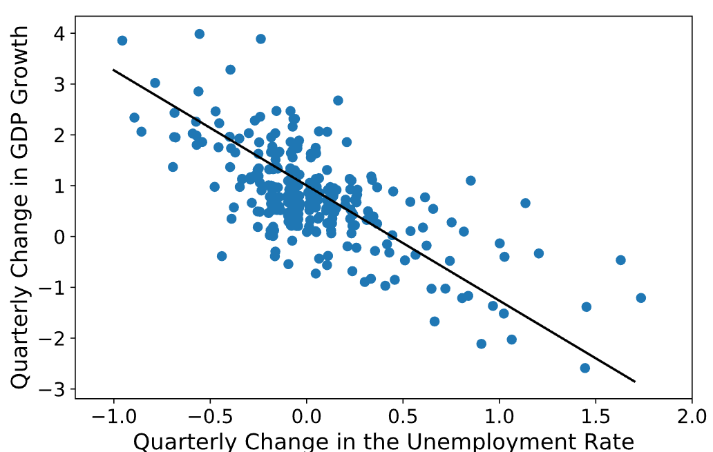
You should also attempt creating the linear regression model to determine its coefficients and intercept. Learn about linear regression here.
Example:
# Create a linear regression model
reg = LinearRegression()# Fit the model to the data
reg.fit(X_train, y_train)# Print the intercept and coefficients
print(reg.intercept_)
print(reg.coef_)
Customizing plots from a figure-level function in Seaborn
The figure-level functions return a FacetGrid instance, which has a few methods for customizing attributes of the plot in a way that is “smart” about the subplot organization. For example, you can change the labels on the external axes using a single line of code:
g = sns.relplot(data=penguins, x="flipper_length_mm", y="bill_length_mm", col="sex")

g.set_axis_labels("Flipper length (mm)", "Bill length (mm)")
While convenient, this does add a bit of extra complexity, as you need to remember that this method is not part of the matplotlib API and exists only when using a figure-level function.
Specifying figure sizes in Seaborn
To increase or decrease the size of a matplotlib plot, you set the width and height of the entire figure, either in the global rcParams, while setting up the plot (e.g. with the figsize parameter of matplotlib.pyplot.subplots()), or by calling a method on the figure object (e.g. matplotlib.Figure.set_size_inches()). When using an axes-level function in seaborn, the same rules apply: the size of the plot is determined by the size of the figure it is part of and the axes layout in that figure.
When using a figure-level function, there are several key differences. First, the functions themselves have parameters to control the figure size (although these are actually parameters of the underlying FacetGrid that manages the figure). Second, these parameters, height and aspect, parameterize the size slightly differently than the width, height parameterization in matplotlib (using the seaborn parameters, width = height * apsect). Most importantly, the parameters correspond to the size of each subplot, rather than the size of the overall figure.
To illustrate the difference between these approaches, here is the default output of matplotlib.pyplot.subplots() with one subplot:
f, ax = plt.subplots()
A figure with multiple columns will have the same overall size, but the axes will be squeezed horizontally to fit in the space:
f, ax = plt.subplots(1, 2, sharey=True)
Facetgrid in Seaborn
In contrast, a plot created by a figure-level function will be square. To demonstrate that, let’s set up an empty plot by using FacetGrid directly. This happens behind the scenes in functions like relplot(), displot(), or catplot():
g = sns.FacetGrid(penguins)
When additional columns are added, the figure itself will become wider, so that its subplots have the same size and shape:
g = sns.FacetGrid(penguins, col="sex")
And you can adjust the size and shape of each subplot without accounting for the total number of rows and columns in the figure:
g = sns.FacetGrid(penguins, col="sex", height=3.5, aspect=.75)
The upshot is that you can assign faceting variables without stopping to think about how you’ll need to adjust the total figure size. A downside is that, when you do want to change the figure size, you’ll need to remember that things work a bit differently than they do in matplotlib.
Relative merits of figure-level functions in Seaborn
Here is a summary of the pros and cons that we have discussed above:
| Advantages | Drawbacks |
| Easy faceting by data variables | Many parameters not in function signature |
| Legend outside of plot by default | Cannot be part of a larger matplotlib figure |
| Easy figure-level customization | Different API from matplotlib |
On balance, the figure-level functions add some additional complexity that can make things more confusing for beginners, but their distinct features give them additional power. The tutorial documentation mostly uses the figure-level functions, because they produce slightly cleaner plots, and we generally recommend their use for most applications. The one situation where they are not a good choice is when you need to make a complex, standalone figure that composes multiple different plot kinds. At this point, it’s recommended to set up the figure using matplotlib directly and to fill in the individual components using axes-level functions.
Combining multiple views on the data -Sample exploratory data analysis
Two important plotting functions in seaborn don’t fit cleanly into the classification scheme discussed above. These functions, jointplot() and pairplot(), employ multiple kinds of plots from different modules to represent multiple aspects of a dataset in a single figure. Both plots are figure-level functions and create figures with multiple subplots by default. But they use different objects to manage the figure: JointGrid and PairGrid, respectively.
Jointplot
jointplot() plots the relationship or joint distribution of two variables while adding marginal axes that show the univariate distribution of each one separately:
sns.jointplot(data=penguins, x="flipper_length_mm", y="bill_length_mm", hue="species")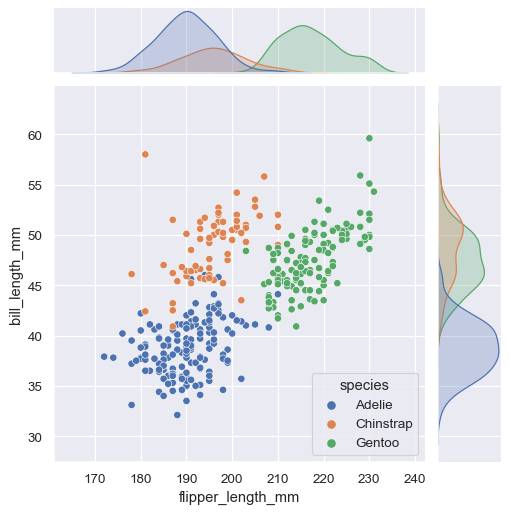
Pairplot
pairplot() is similar — it combines joint and marginal views — but rather than focusing on a single relationship, it visualizes every pairwise combination of variables simultaneously:
sns.pairplot(data=penguins, hue="species")
Behind the scenes, these functions are using axes-level functions that you have already met (scatterplot() and kdeplot()), and they also have a kind parameter that lets you quickly swap in a different representation:
sns.jointplot(data=penguins, x="flipper_length_mm", y="bill_length_mm", hue="species", kind="hist")
Advantages of Data Visualization using Python
Data visualization generally enhances understanding, promotes collaboration, and facilitates informed decision-making, thus making it a valuable tool for data analysis and communication. Review the following advantages of data visualization:
- Improved Understanding: Visual representations of data make complex information easier to comprehend and interpret.
- Insight Discovery: Visualizations can reveal patterns, trends, and relationships that may not be apparent in raw data, leading to new insights and discoveries.
- Effective Communication: Visualizations facilitate clear and concise communication of data insights to stakeholders, helping to convey messages more effectively than raw data or text alone.
- Decision Making: Visualizations enable informed decision-making by providing stakeholders with actionable insights and evidence-based recommendations.
- Increased Engagement: Engaging and visually appealing graphics capture attention and encourage interaction with the data, fostering greater engagement and understanding.
- Efficient Analysis: Visualizations streamline the data analysis process by allowing users to quickly identify relevant information and focus on key areas of interest.
- Collaboration: Visualizations promote collaboration among team members by providing a common understanding of the data and facilitating discussions and brainstorming sessions.
Reference and further reading for data visualization with Python, Matplotlib and Seaborn
Matplotlib Cheatsheet: https://matplotlib.org/cheatsheets/_images/cheatsheets-1.png
Seaborn Cheatsheet: https://s3.amazonaws.com/assets.datacamp.com/blog_assets/Python_Seaborn_Cheat_Sheet.pdf
Frequently Asked Questions about data visualization with Python, Matplotlib and Seaborn
What is data visualization in Python?
Data visualization in Python refers to the process of creating graphical representations of data using Python plotting libraries. It helps in understanding data patterns, trends, and relationships by displaying data in forms such as plots, charts, and graphs. Popular libraries for data visualization in Python include Matplotlib, Seaborn, Plotly, and Bokeh. These tools offer a range of customization options to create informative and visually appealing visualizations.
Is Python good for data Visualization?
Yes, Python is excellent for data visualization. With libraries like Matplotlib, Seaborn, Plotly, and Bokeh, Python provides powerful tools for creating a wide range of visualizations. These libraries offer flexibility, interactivity, and a variety of plotting options, making Python a popular choice for data visualization tasks. Additionally, Python’s simplicity and ease of use make it accessible to beginners while also providing advanced features for more experienced users.
What are the basic principles of data visualization?
The basics key principles of data visualization involve tailoring visualizations to the audience, choosing appropriate chart types (e.g., bar, line, scatter, histograms, pie), simplifying visuals, using appropriate scales and clear labeling, using color effectively, highlighting key points, maintaining proportions, considering accessibility, and telling a compelling story with the data. These principles help create effective and engaging visualizations that communicate data insights effectively.
What are the advantages of data visualization?
Data visualization offers several advantages such as enhanced comprehension of complex information, discovery of patterns and trends in data, clear communication of insights to stakeholders, support for informed decision-making, increased engagement through visually appealing graphics, streamlined data analysis process, and promotion of collaboration among team members.
What is meant by exploratory data analysis (EDA)?
Exploratory Data Analysis (EDA) refers to the process of analyzing datasets to summarize their main characteristics, often using visual methods. It involves:
– Understanding Data Structure: Identifying data types, dimensions, and structures.
– Detecting Outliers and Anomalies: Finding unusual data points.
– Identifying Patterns and Relationships: Using visualizations to uncover trends and correlations.
– Summarizing Data: Computing summary statistics like mean, median, and standard deviation.
– Checking Assumptions: Verifying assumptions for statistical models.What is EDA used for?
Exploratory Data Analysis (EDA) is used for:
– Understanding Data: Getting an initial sense of the data’s structure, quality, and key characteristics.
– Detecting Anomalies: Identifying outliers, missing values, and errors.
– Finding Patterns and Relationships: Discovering trends, correlations, and potential causal relationships.
– Guiding Further Analysis: Informing the selection of appropriate statistical models and analysis techniques.
– Generating Hypotheses: Formulating questions and hypotheses for deeper investigation.What are the steps of EDA (exploratory data analysis)?
The steps of Exploratory Data Analysis (EDA) typically include:
– Data Collection: Gathering the relevant data from various sources.
– Data Cleaning: Handling missing values, correcting errors, and dealing with outliers.
– Data Profiling: Summarizing the main characteristics of the data using descriptive statistics.
– Data Visualization: Creating plots and charts to visualize the data distributions, trends, and relationships.
– Feature Engineering: Creating new features or transforming existing ones to improve analysis.
– Hypothesis Testing: Conducting preliminary statistical tests to identify significant patterns or relationships.
– Insights and Reporting: Documenting findings and insights for further analysis or decision-making.What is Matplotlib?
Matplotlib is a Python library used for creating static, animated, and interactive visualizations in Python.
How do you create a simple plot using Matplotlib?
You can create a simple plot using Matplotlib by calling the
plotfunction and passing the data to be plotted.What are the components of a Matplotlib Figure?
The components of a Matplotlib Figure include the Figure itself, Axes, Axis, and Artists.
How do you create a Figure with multiple Axes?
You can create a Figure with multiple Axes using
plt.subplots()and specifying the desired number of rows and columns.What is the difference between the object-oriented (OO) style and the pyplot style in Matplotlib?
In the object-oriented (OO) style, you explicitly create Figures and Axes objects and call methods on them, while in the pyplot style, you rely on
pyplotto manage Figures and Axes automatically.What are some advantages of using the object-oriented style in Matplotlib?
The object-oriented style offers more control and flexibility, making it suitable for complex plots and reusable code.
What types of inputs do Matplotlib plotting functions expect?
Matplotlib plotting functions expect numpy arrays or objects that can be converted to arrays using
numpy.asarray.What is Seaborn in data visualization?
Seaborn is a Python visualization library based on Matplotlib that provides a high-level interface for drawing attractive and informative statistical graphics.
How do you import Seaborn?
Seaborn can be imported using the statement
import seaborn as sns.What is the purpose of pairplot in Seaborn?
The purpose of
pairplotin Seaborn is to visualize pairwise relationships between variables in a dataset, displaying scatterplots for continuous variables and histograms for the marginal distributions.How do you customize the appearance of plots created with Seaborn?
You can customize the appearance of plots created with Seaborn using various parameters and attributes provided by the plotting functions, such as
hue,size, andstyle.What is the advantage of using figure-level functions in Seaborn?
Figure-level functions in Seaborn offer easy faceting by data variables and provide a unified interface for customizing plots across multiple subplots.
What are the advantages of seaborn?
High-Level Interface: Seaborn offers a high-level interface for creating complex statistical visualizations with minimal code, making it easier to generate sophisticated plots compared to Matplotlib.
Attractive Defaults: Seaborn comes with attractive default styles and color palettes, allowing users to create visually appealing plots without manual customization.
Statistical Visualization: Seaborn is specifically designed for statistical data visualization, providing specialized functions for exploring relationships between variables, visualizing distributions, and identifying patterns in data.
Integration with Pandas: Seaborn seamlessly integrates with pandas data structures, enabling users to directly visualize datasets loaded into pandas DataFrames without preprocessing.
Faceting and Grids: Seaborn offers convenient functions for creating grid-based plots and faceted visualizations, allowing users to explore multiple aspects of their data simultaneously.How do you specify figure sizes in Seaborn?
Figure sizes in Seaborn can be specified using parameters like
heightandaspectin figure-level functions, which control the size and shape of each subplot.Can you combine multiple views of data in a single figure using Seaborn?
Yes, you can combine multiple views of data in a single figure using Seaborn’s
jointplotandpairplotfunctions, which display joint distributions and marginal distributions simultaneously.What is the difference between Matplotlib and Seaborn?
Matplotlib is a foundational Python library used for creating a wide range of static, animated, and interactive visualizations. It offers extensive control over plot elements and is highly customizable. However, it can be verbose and requires more code to achieve aesthetically pleasing plots.
Seaborn, on the other hand, is built on top of Matplotlib and provides a high-level interface for drawing attractive and informative statistical graphics with less code. Seaborn is specifically designed for statistical visualization and comes with built-in themes and color palettes, making it easier to produce visually appealing and informative plots. It also integrates well with pandas data structures, simplifying the process of working with datasets.