Dive into supervised machine learning with these straightforward steps. Learn how to use models leveraging labeled data to make accurate predictions and classifications. Perfect for beginners looking to understand and implement supervised learning effectively.
Machine learning is important because it gives enterprises a view of trends in customer behavior and business operational patterns, as well as supports the development of new products. Many of today’s leading companies, such as Meta, Google, Netflix and Uber, make machine learning a central part of their operations. Machine learning has become a significant competitive differentiator for many companies.
What are common ways in which machines learn?
Classical machine learning is often categorizes algorithms in the way it learns and predicts accurately. There are four basic approaches: supervised learning, unsupervised learning, semi-supervised learning / self-supervised learning and reinforcement learning. The type of algorithm data scientists choose to use depends on what type of data they want to predict.
Supervised learning
In this type of machine learning, data scientists supply algorithms with labeled training data and define the variables they want the algorithm to assess for correlations. Both the input and the output of the algorithm is specified.
Unsupervised learning
This type of machine learning involves algorithms that train on unlabeled data. The algorithm scans through data sets looking for any meaningful connection. The data that algorithms train on are predetermined while the predictions or recommendations they output are learned from the data.
Semi-supervised learning
This approach to machine learning involves a mix of the two preceding types. Data scientists may feed an algorithm mostly labeled training data, but the model is free to explore the data on its own and develop its own understanding of the data set.
Reinforcement learning
Data scientists typically use reinforcement learning to teach a machine to complete a multi-step process for which there are clearly defined rules. Data scientists program an algorithm to complete a task and give it positive or negative cues as it works out how to complete a task. But for the most part, the algorithm decides on its own what steps to take along the way.
Introduction to supervised machine learning
Supervised machine learning is a type of artificial intelligence that trains algorithms on labeled data to make predictions or take actions based on input data. It involves a model learning from past observations and making predictions on new, unseen data. The goal is to develop a model that can generalize from the training data to unseen data.
Supervised machine learning is a subfield of artificial intelligence where a model is trained on labeled data to make predictions or take actions based on new input data. It uses algorithms that can learn from the data and improve their predictions over time. The labeled data used in supervised learning includes input features and corresponding output labels, allowing the algorithm to learn the relationship between the inputs and outputs. This learning process helps the algorithm make accurate predictions on new data it has not seen before.
Supervised learning is used in a wide range of applications, such as image classification, speech recognition, sentiment analysis, and predictive maintenance. The success of a supervised learning model depends on the quality and size of the training data, as well as the choice of algorithm. Common algorithms used in supervised learning include linear regression, logistic regression, decision trees, and neural networks.
What is supervised learning?
As the name suggests, supervised learning involves training a computer system using labeled data. This means that each piece of data comes with a known correct answer. The system learns from these examples to make predictions or classifications on new, unlabeled data. Essentially, the machine is taught using a set of training examples, which it uses to analyze and accurately predict outcomes for new data.

In this instance, we have pictures labeled as “spoon” or “knife”. The machine receives this known data and processes it to assess and learn the correlation of the images based on their characteristics, such as size, shape, sharpness, etc. Now, using the historical data, the machine can properly predict that a fresh image fed to it is a spoon based on its characteristics. Thus, the machine learns the things from training data and then applies the knowledge to test data.
Supervised machine learning requires the data scientist to train the algorithm with both labeled inputs and desired outputs. Supervised learning algorithms are good for the following tasks:
- Binary classification: Dividing data into two categories.
- Multi-class classification: Choosing between more than two types of answers.
- Regression modeling: Predicting continuous values.
- Ensembling: Combining the predictions of multiple machine learning models to produce an accurate prediction.
Supervised learning is classified into two categories of algorithms:
- Classification
- Regression
Want to get into a machine learning career? Read this post or enroll in our machine learning work experience program.
-
 Machine Learning Engineer Work Experience Certification Course ProgramProduct on sale₹69,999

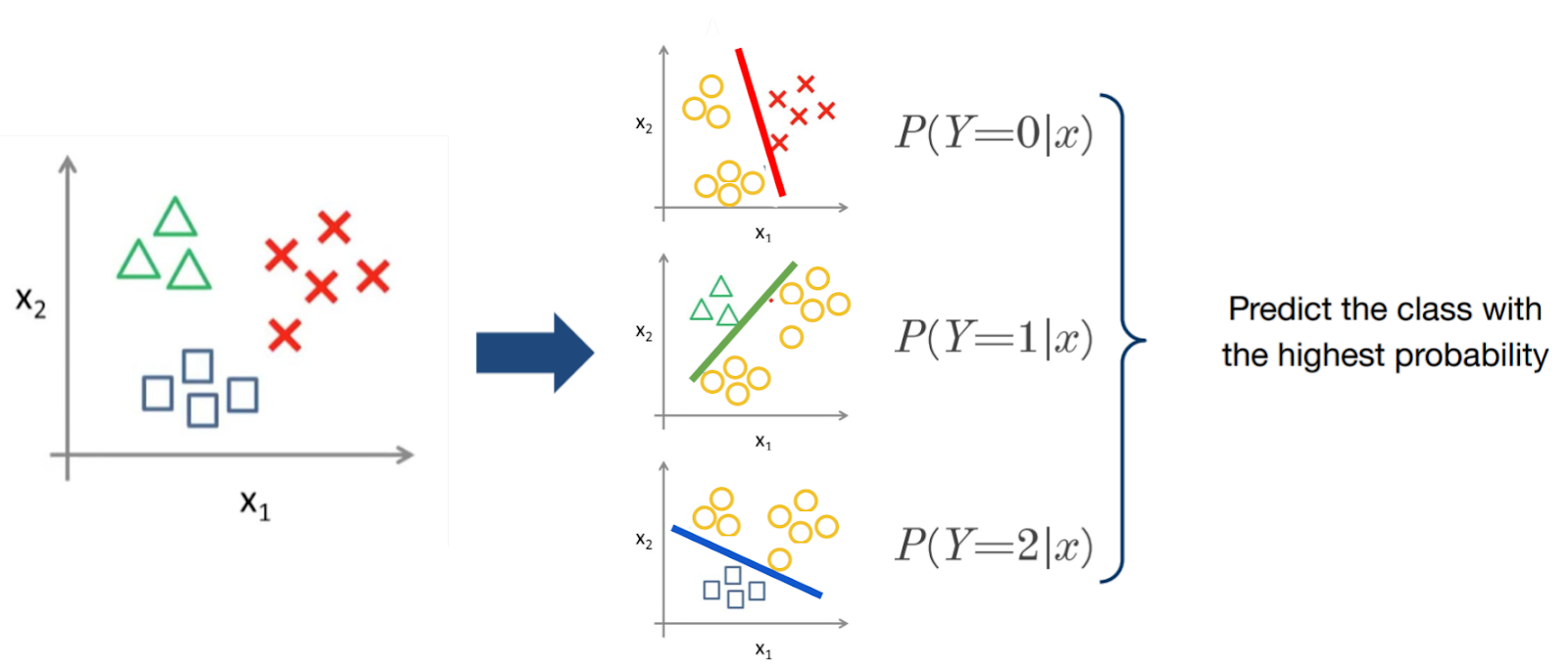
Introduction to classification as a supervised learning technique
Classification is a type of supervised machine learning where the model is trained to predict a categorical output. The output can be one of several pre-defined classes. It’s used for problems like spam detection, sentiment analysis, and image classification. The model is trained to learn the relationship between input features and the output class, allowing it to make predictions for new data.
The variable to be predicted has two or more classes and is categorical, say, true or false, male or female, yes or no, etc.
For example, to determine if an email is spam, we first need to train the computer to recognize what spam looks like. This is done by using spam filters that analyze the email’s header and body for suspicious patterns. These filters look for specific keywords and check against known blacklists of banned spammers. Based on these factors, the email is assigned a spam score. A lower spam score indicates a lower likelihood of the email being spam. The algorithm then uses this score, along with the content and labels, to decide whether new incoming emails should be placed in the inbox or the spam folder.

Get started immediately with classification using KNN – python example with scikit learn
from sklearn.datasets import load_digits
from sklearn.model_selection import train_test_split
from sklearn.neighbors import KNeighborsClassifier
from sklearn.metrics import accuracy_score

# Load the digits dataset
digits = load_digits()
X = digits.data
y = digits.target

# Split the data into training and testing sets
X_train, X_test, y_train, y_test = train_test_split(X, y, test_size=0.3, random_state=42)

# Create and train the K-Nearest Neighbors classifier
model = KNeighborsClassifier()
model.fit(X_train, y_train)

# Make predictions
y_pred = model.predict(X_test)

# Evaluate the model
accuracy = accuracy_score(y_test, y_pred)
print(f"Accuracy: {accuracy:.2f}")
Introduction to regression as a supervised learning technique
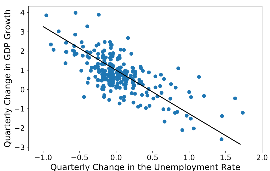
Regression is a type of supervised machine learning that involves predicting a continuous output value. It’s used for problems like stock price prediction, housing price prediction, and weather prediction. The model is trained to learn the relationship between input features and the output value, allowing it to make predictions for new data.
The variable to be predicted is a real or continuous value. A change in one variable is related to a change in the other in this situation because there is a relationship between the two or more variables. For instance, regression can be used to predict the house price from training data that may include locality, size of a house, etc.
Regression example with simple explanation
Let’s take two variables: temperature and humidity. The independent variable in this situation is “temperature,” and the dependent variable is “humidity.” The humidity drops as the temperature rises.
The model is fed these two variables, and as a result, the computer learns how they relate to one another. Once trained, the system can accurately forecast the humidity depending on the temperature.
The following is another example of airfare vs distance.

Get started immediately with linear regression – python example with scikit learn
import numpy as np
from sklearn.datasets import load_diabetes
from sklearn.linear_model import LinearRegression
from sklearn.model_selection import train_test_split
from sklearn.metrics import mean_squared_error

# Load the diabetes dataset
diabetes = load_diabetes()
X = diabetes.data
y = diabetes.target

# Split the data into training and testing sets
X_train, X_test, y_train, y_test = train_test_split(X, y, test_size=0.2, random_state=42)

# Create and train the linear regression model
model = LinearRegression()
model.fit(X_train, y_train)

# Make predictions
y_pred = model.predict(X_test)

# Evaluate the model
mse = mean_squared_error(y_test, y_pred)
print(f"Mean Squared Error: {mse:.2f}")
Applications of supervised learning
- Risk Assessment: In order to reduce the risk portfolio of the companies, supervised learning is used to analyze risk in the financial services or insurance domains.
- Image classification: One of the primary use cases for showing supervised machine learning is image categorization. For instance, Facebook can identify your friend in a photo from a collection of tagged images.
- Fraud Detection: To determine whether the user’s transactions are genuine or not.
- Visual Recognition: The capacity of a machine learning model to recognize images, actions, places, people, and things.
Advantages: –
- Supervised learning allows collecting data and produces data output from previous experiences.
- Helps to optimize performance criteria with the help of experience.
- Supervised machine learning helps to solve various types of real-world computation problems.
Disadvantages: –
- Classifying big data can be challenging.
- Training for supervised learning needs a lot of computation time. So, it requires a lot of time.
-
Machine Learning Engineer Work Experience Certification Course ProgramProduct on sale₹69,999
Classification vs regression
Classification and regression are two types of supervised machine learning that are used to solve different types of problems. In classification, the goal is to predict a categorical output, while in regression, the goal is to predict a continuous output. The choice between the two depends on the nature of the problem and the type of output required.
Classification and regression are two common types of supervised machine learning. The main difference between them is the type of output they predict.
- Classification is a type of supervised machine learning that is used to predict a categorical output, such as a label or a class. The output can be one of several pre-defined classes, and the goal is to train a model that can accurately predict the class of new, unseen data. Examples of classification problems include image classification, spam detection, and sentiment analysis.
- Regression, on the other hand, is used to predict a continuous output, such as a numerical value. The goal is to train a model that can accurately predict the value of a continuous target variable based on input features. Examples of regression problems include stock price prediction, housing price prediction, and weather prediction.
The choice between classification and regression depends on the nature of the problem and the type of output required. If the goal is to predict a categorical output, then classification is the appropriate technique. If the goal is to predict a continuous output, then regression is the appropriate technique.
How to decide when to use regression or classification models?
| Aspect | Regression Models | Classification Models |
|---|---|---|
| Objective | Predict a continuous numeric value. | Predict a discrete label or category. |
| Output | Continuous (e.g., real numbers). | Categorical (e.g., class labels). |
| Examples | – Predicting house prices based on features like size and location. – Estimating a person’s weight based on height and age. – Forecasting sales revenue for the next quarter. | – Classifying emails as spam or not spam. – Diagnosing a disease based on patient symptoms. – Identifying whether a customer will buy a product or not. |
| Typical Algorithms | – Linear Regression – Polynomial Regression – Ridge/Lasso Regression – Support Vector Regression (SVR) | – Logistic Regression – Decision Trees – Random Forests – Support Vector Machines (SVM) – k-Nearest Neighbors (k-NN) |
| Evaluation Metrics | – Mean Absolute Error (MAE) – Mean Squared Error (MSE) – Root Mean Squared Error (RMSE) – R-squared (R²) | – Accuracy – Precision – Recall – F1 Score – Confusion Matrix |
| Use Case Considerations | Regression is used when the outcome variable is continuous and the goal is to predict exact values or quantities. | Classification is used when the outcome variable is categorical, and the goal is to categorize or label inputs into discrete classes. |
| Visual Representation | Typically involves plotting a continuous line or surface against the data points in a scatter plot. | Typically involves plotting boundaries or regions that separate different classes in a feature space. |
Reference and further reading about supervised learning
- Outliers: Finding Them in Data, Formula, Examples. Easy Steps and Video – Statistics How To
- ML-powered anomaly detection for outliers – Amazon QuickSight
- https://www.section.io/engineering-education/complete-guide-to-dealing-with-missing-values-in-python
Frequently Asked Questions About Supervised Learning in Machine Learning
What is the difference between supervised and unsupervised learning?
Supervised learning uses labeled data to train models, aiming to predict outcomes or classify data based on known inputs. Unsupervised learning works with unlabeled data, seeking to identify patterns, groupings, or structures without predefined categories.
What are the two 2 types of supervised learning?
The two types of supervised learning are regression, which predicts continuous values, and classification, which predicts discrete categories.
What is an example of supervised machine learning?
An example of supervised machine learning is predicting house prices using a dataset with labeled features (e.g., size, location) and known prices.
What is an example of supervised machine learning classification?
An example of supervised machine learning classification is email spam detection, where the model classifies emails as “spam” or “not spam” based on labeled training data.
Why is supervised learning called so?
Supervised learning is called so because the model is trained on labeled data, with the “supervision” coming from the known input-output pairs that guide the learning process.
What is an example of unsupervised learning?
Real-world applications of unsupervised learning include:
– Customer Segmentation: Grouping customers based on purchasing behavior to tailor marketing strategies.
– Anomaly Detection: Identifying unusual patterns, such as fraud detection in financial transactions.
– Recommendation Systems: Discovering patterns in user preferences to suggest products or content, as seen in streaming services.
– Topic Modeling: Extracting topics from large collections of text, like summarizing customer reviews or academic papers.Is ChatGPT supervised or unsupervised?
ChatGPT is primarily trained using unsupervised learning / self-supervised techniques, where it learns patterns and language structures from large amounts of text data without specific labels or supervision. However, fine-tuning may involve supervised learning, where the model is further trained on a dataset with labeled examples to improve performance on specific tasks or align responses with desired behavior.
Is a decision tree supervised or unsupervised?
A decision tree is a supervised learning algorithm. It is used for both classification and regression tasks, where it learns from labeled data to make predictions or decisions based on input features.
What is another name for supervised learning?
Another name for supervised learning is “labeled learning” or “controlled learning” or “supervised machine learning”.
Is KNN supervised or unsupervised?
K-Nearest Neighbors (KNN) is a supervised learning algorithm. It classifies or predicts the label of a data point based on the labels of its nearest neighbors in the training dataset.
What is the main goal of supervised learning?
The main goal of supervised learning is to train a model to make accurate predictions or classifications based on labeled input-output pairs, using known data to learn patterns that can be applied to new, unseen data.
What is the disadvantage of supervised learning?
A disadvantage of supervised learning is that it requires a large amount of labeled data, which can be time-consuming and expensive to obtain. Additionally, the model’s performance is limited by the quality and representativeness of the training data.
What example uses supervised learning?
Supervised learning is used in a variety of applications, including:
Spam Detection: Classifying emails as spam or not spam.
Image Classification: Identifying objects or features in images.
Medical Diagnosis: Predicting diseases based on patient data.
Speech Recognition: Translating spoken language into text.
Fraud Detection: Identifying fraudulent transactions in financial systems.
Predictive Analytics: Forecasting future trends, such as sales or stock prices.